Site relevance: how to replicate Google’s siteRadius and siteFocusScore with embeddings

In the quality post I listed some of the signals that Google stores at site level. Two of them stuck with me: siteFocusScore, how focused a site is on one topic, and siteRadius, how far its pages drift from that central topic.

Recently I had to analyse a B2B SaaS that wanted to rank a new product and could not get it to move. It had pages and internal links, and the product barely showed up on Google. I used it as an excuse to replicate those two metrics with an embeddings model that runs on a laptop, with no GPU and no paid APIs.

Everything is in this post: what Google stores, which patents and papers are behind it, how I calculated it step by step, the code, what came out and its limits. It won’t give you Google’s number, but it works as a proxy to visualise the relevance of your site. The data in the example is anonymised. The products are called A, B, C and “the new product”, and the competitors are 1, 2 and 3.

What is site relevance?

When we talk about relevance we almost always think about the page: whether it answers the search, whether it has the right entities, whether the title fits. That still holds. But Google also looks at the whole site. It says so in its guide to ranking systems, and it announced it in 2022 with the helpful content update:

That system no longer works on its own: since March 2024 it has been part of the core ranking systems, and the guide lists it among the retired ones. The idea of site-level signals is still in the current guide, which is the first quote.

That 2022 post came with a list of questions for self-assessment, such as “Does your site have a primary purpose or focus?”, and another list of warning signs, including “Are you producing lots of content on different topics in hopes that some of it might perform well in search results?”. The current documentation keeps both (it now says “many different topics”).

Be careful not to read that as “one site, one topic”. Danny Sullivan clarified it soon after, and John Mueller used the same idea when reviewing a website that had lost traffic and indexing:

A site can have several topics. Sullivan explained it in the next message: what counts is the “in hopes that some of it might perform well” part, opening up topics to see if any of them works.

For this post, the relevance of a site is how well each page fits with what the site is about. And that can be measured with vectors.

What does Google store?

In the May 2024 Content Warehouse API leak there is a module dedicated to this, QualityAuthorityTopicEmbeddingsVersionedItem:

Field	Description in the leak
pageEmbedding	No description
siteEmbedding	“Compressed site/page embeddings.”
siteFocusScore	“Number denoting how much a site is focused on one topic.”
siteRadius	“The measure of how far page_embeddings deviate from the site_embedding.”
versionId	No description

In other words: one vector per page, one vector per site, one number for focus and another for how far the pages sit from the centre.

The module isn’t isolated. It appears inside CompressedQualitySignals, the package of compressed signals that Google stores with each document, in the topicEmbeddingsVersionedData field: “Versioned TopicEmbeddings data to be populated later into superroot / used directly in scorers”. The systems that score (scorers) use them directly, or they are passed later to superroot, the layer that reorders and assembles the results.

The documentation for that package says where it lives: in Mustang, the main ranking system, and in TeraGoogle, the secondary index. In TeraGoogle it goes with each document’s data, “which means it can be used in preliminary scoring”, the first screening of candidates, and in a memory that the documentation itself describes as “very limited”. The embeddings share a package with siteAuthority, the site’s authority, and babyPandaV2Demotion, a demotion applied on top of Panda.

My reading: Google doesn’t spend scarce memory on something it doesn’t use. These embeddings are attached to each URL, next to known ranking signals, and are available at scoring time.

There is another module that fits, QualityNsrNsrData, with the site-level quality signals (NSR). Three things in it are relevant to this post:

• Another vector per site. site2vecEmbedding: “Site2vec embeddings”. Its compressed version is “to be used in superroot since the full embeddings take too much space”.
• What a site is for Google. siteChunk: “Primary NSR sitechunk”. It almost always matches the host of the canonical URL, but “in rare, but important cases” it is calculated from the page markup, and there is an even finer secondarySiteChunk. A site can be a piece of your domain.
• How much quality varies between pages. siteQualityStddev is the dispersion of the quality scores (PQ) of a site’s pages, and chardScoreVariance, the variance of chard, a “site quality predictor based on content”.

That last one seems important to me: besides the mean, Google stores how spread out a site’s pages are. On topic, with siteRadius. On quality, with these two fields.

Mike King read it this way in his analysis of the leak: Google may be “comparing the page embeddings to the site embeddings to see how off-topic the page is”.

The leak is a data schema. It doesn’t say how those fields are calculated or how much they weigh, and Google, through Davis Thompson, asked people not to draw conclusions “based on out-of-context, outdated, or incomplete information”. Everything from here on replicates the idea with public tools. The value Google calculates can’t be seen from the outside.

What do the patents say?

Before going through them one by one, here is the map: 25 years of papers, Google patents and Google documentation on site-level relevance.

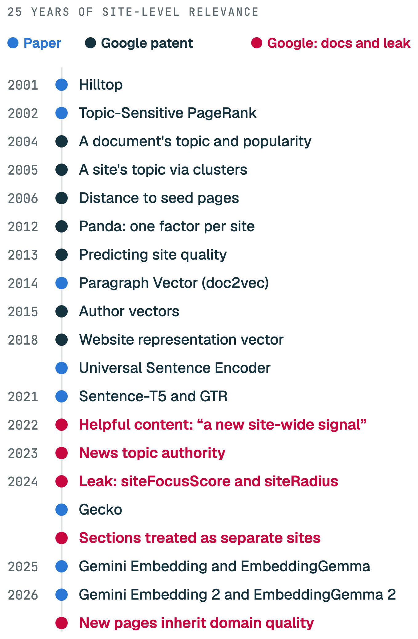
The closest is Website representation vector, filed in 2018 and abandoned in the United States. It describes a neural network that turns the content of a site (text, images and links) into a vector. It then groups sites by “a quality score representing a quality measure of the website relative to other websites”, combines the vectors of each group “by averaging, multiplying, summing, or dividing” and classifies a new site by how close it sits to each group. It does this by area of knowledge, and the example groups are sites written by experts (doctors), apprentices (medical students) and laypeople. Bill Slawski analysed it in 2020, before the leak.

Note that this patent groups sites by quality. The mechanics, though, are the same ones we are going to use: content vectors, a mean as the centre and distances to that centre.

The idea of getting a site’s topic by clustering its content is much older. In 2005 Google filed a patent (granted in 2012 and now expired) to categorise a website from clusters of its content: it calculates “a set of scored clusters (e.g., semantic, term co-occurrence, etc.) for the Website” and maps them to a taxonomy.

Then there are the Panda ones, which I already covered in the quality post. Here I’ll stick with another one by Navneet Panda with the same title, Ranking search results: it groups results by domain and applies “a group-based modification factor” to each result in the group. It is the clearest way of saying that a site score changes how each page ranks. The other two, Site quality score and Predicting site quality, calculate that score from the searches that refer to the site (branded) compared with those that end in a click on it, or from the language of the site.

There is a link-based version of the same idea. The patent on distances in the link graph, by Nissan Hajaj, “computes shortest distances from the set of seed pages to each page” and ranks with those distances. The space changes (links instead of text), but it still measures how far you are from a centre. That is why, further down, I also calculate the site centre weighted by internal PageRank.

And a curious one: Generating author vectors, by Brian Strope and Quoc Le, trains one vector per author from what they write and can group them. Quoc Le is a co-author of Paragraph Vector, the paper that popularised document vectors, and Strope is one of the authors of the Universal Sentence Encoder. The names on the vector patents are the same ones on the papers.

Be careful with two patents that are often cited for this and don’t say what’s attributed to them. Ranking search results based on entity metrics has no site-level authority metric. And Determining topic authority scores authors within a collection of documents, without mentioning websites or search results. And, as always, something being patented doesn’t mean it’s in use.

And the papers?

The topical relevance of a site has roots in two papers from the early 2000s. Hilltop (2001), by Krishna Bharat, who ended up at Google, ranks through “expert” pages on a topic. Topic-Sensitive PageRank (2002), by Taher Haveliwala, calculates “a set of PageRank vectors, biased using a set of representative topics”. Both mix topic and authority.

The vector side has a clear lineage inside Google:

Year	Paper	What it adds
2014	Paragraph Vector (Le and Mikolov)	A fixed-size vector for a whole document
2018	Universal Sentence Encoder	General embeddings for sentences and short texts
2021	Sentence-T5 and GTR	T5-based embeddings and retrieval with two encoders
2024	Gecko	Compact embeddings distilled from an LLM
2025	Gemini Embedding	The first embeddings model based on Gemini
2025	EmbeddingGemma	A small, open model you can run locally
2026	Gemini Embedding 2	Google’s current model, multimodal: text, image, video, audio and documents in the same space
2026	EmbeddingGemma 2	The open, multimodal version, which also runs locally

Outside Google, Homepage2Vec (EPFL, 2022) already made one vector per website to classify its topic in 92 languages. And a 2025 benchmark comparing ways of building website vectors found that text matters most, and that TF-IDF with a small network competes well. You don’t need the biggest model to measure this.

I used multilingual-e5-small, from Microsoft (E5 paper and multilingual version). It has 384 dimensions, covers about 100 languages and runs on CPU. The model card says three things that matter for this calculation:

1. It truncates at 512 tokens. If you give it a whole page, it only reads the start. That’s why I split each page into chunks.
2. You have to add the query: prefix when you use the vectors for clustering or as features.
3. Cosines are concentrated between 0.7 and 1.0. Distances come out tiny (0.03) and can only be compared between sites processed with the same model and the same preprocessing.

And a general warning: a Netflix paper, Is Cosine-Similarity of Embeddings Really About Similarity?, shows that with some embeddings the cosine can give similarities that are “arbitrary and therefore meaningless”. With models trained for similarity, like E5, it works, but it is good to know before treating the number as truth.

How is it calculated?

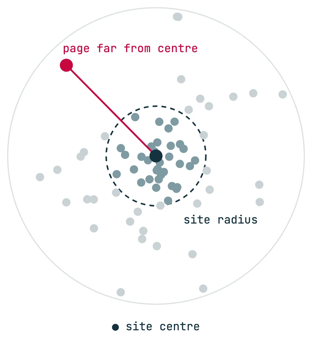
The mechanics fit in five lines:

• Page vector: the mean of the vectors of its text chunks.
• Site centre: the mean of the page vectors, normalised.
• Distance: 1 minus the cosine between the page and the centre.
• Site radius: the mean distance of the pages.
• Outside the radius: a page that is further away than that mean.

This is how I did it, step by step.

1. Crawl and keep the text that matters

I crawled the indexable pages that return 200 and are their own canonical, and extracted the text from headings, paragraphs, lists and tables. You have to remove everything that repeats on every page: menu, footer, banners. Otherwise all the pages look alike because they share the same footer.

My rule: a block of text that appears on more than 30% of pages is boilerplate and goes. Note that if a page type has more than 30% of your URLs, its template text goes too. To keep it, raise the threshold above your biggest page type’s share of URLs or count the frequency within each page type. In the example, that rule removed 119 blocks.

# rows: the crawled pages; blocks_of(row): its text blocks
counts = defaultdict(int)
for row in rows:
    for block in set(blocks_of(row)):
        counts[block] += 1
boilerplate = {block for block, c in counts.items() if c / len(rows) > 0.3}

2. One vector per page

I cut each page into chunks of 180 words and keep the first 8, about 1,440 words. Both figures are optimisation decisions. The crawl already gave me the word count of each page, with the median at 1,016, so with 8 chunks most pages fit whole, and the cut stops very long ones, like one with 18,000 words, from blowing up the calculation time. And although the model accepts up to 512 tokens, I limit it to 256, where the 180-word chunks fit, because it’s faster that way. With these two adjustments the calculation runs on a normal laptop, with no GPU: you don’t need a powerful computer to do it with your site. I calculate the vector of each chunk, take the mean and normalise it. That is the page vector.

model = SentenceTransformer('intfloat/multilingual-e5-small', device='cpu')
model.max_seq_length = 256
# pieces: the chunks of all the pages; owner: which page each chunk belongs to
chunk_vectors = model.encode(['query: ' + piece for piece in pieces], normalize_embeddings=True)
owner = np.array(owner)
vectors = np.stack([chunk_vectors[owner == i].mean(0) for i in range(n_pages)])
vectors /= np.linalg.norm(vectors, axis=1, keepdims=True)

In the example, 2,035 pages in English gave 12,636 chunks.

I don’t process the translations. Each translation inherits the vector of its English original through hreflang. That has one advantage: the model is multilingual, but it still places the same text in two languages at slightly different points, and that would add language noise. And it has a cost worth being clear about: this way the radius can’t see whether a translation is bad.

3. The site centre and the distance of each page

w = weights / weights.sum()
mean = (vectors * w[:, None]).sum(0)
focus = np.linalg.norm(mean)       # 1 if all pages point the same way
site = mean / focus                # the site centre
distance = 1 - vectors @ site      # 1 - cosine with the centre
radius = (distance * w).sum()      # mean distance: the radius
outside = distance > radius

Since absolute distances cannot be compared between models, I convert each distance to a percentile by rank, from 0 (the page closest to the centre) to 1 (the furthest). In the tables I show it from 0 to 100. And for each page type I look at two things, the percentage of pages outside the radius and their median percentile.

4. Decide how much each page weighs

The centre depends on how you weight the pages, and that decision changes the result a lot. I tried three versions on the more than 14,000 URLs of the site, counting translations:

Median percentile	Every URL equal	By internal PageRank	By estimated traffic
Product B	9	17	28
Product C	27	56	12
Product A	39	23	47
Free tools	62	59	64
New product	80	21	83
Blog	85	67	87
Site radius	0.0286	0.0321	0.0128

Each version is good for reading something different. If every URL weighs the same, the page types with many near-identical pages dominate. Weighted by traffic, product C takes 78% of the weight and pulls the centre towards itself. Weighted by internal PageRank, the new product jumps from the 80th to the 21st percentile, because its pages receive 11% of the internal PageRank.

Together, the equal-weight and PageRank versions tell you what’s happening to the new product. Internal linking passes it authority, and yet, when every URL weighs the same, its content sits far from the centre. The links reach it; what fails is the relevance of its pages, and that fits with it barely showing up on Google. We look at it in more detail in the example.

Which one does Google use? We don’t know. For the diagnosis I stick with “every URL equal”: the leak says nothing about weights, and it is how tools like Screaming Frog calculate the centre. I use the other two to understand what pulls on the centre.

5. Name the topics

To know what the centre is about, I built one vector per topic with the 60 highest-volume keywords of each product and looked at which topic each page resembles. Ten years ago, in the industry, this was done with TF-IDF and LSI keywords, an approach that is quite outdated today: TF-IDF counts words and embeddings compare meanings.

Here you can see the E5 compression I mentioned earlier. The vectors of the five topics have cosine similarities of 0.90 to 0.94 with each other, even though they are different products. With these models, anything that talks about a similar industry ends up close. That’s why I work with percentiles.

6. Draw it without lying

A 2D map of 384-dimensional vectors always distorts something. PCA or t-SNE distort exactly what I want to show, the distance to the centre. So I separated the two things:

• The order of distances is real. Each page is placed at its percentile of distance to the centre: you can see which pages are further away, though not by how much.
• The angle only groups. I project what separates each page from the centre onto the plane that best separates the topics: the first two components of the category centres.

cats = np.array(cats)
categories = np.unique(cats)
# what pulls each page away from the centre
offsets = vectors - np.outer(vectors @ site, site)
# the plane that best separates the category centres
means = np.stack([offsets[cats == c].mean(0) for c in categories])
_, _, vt = np.linalg.svd(means - means.mean(0), full_matrices=False)
xy = offsets @ vt[:2].T
# the direction only groups; the map radius is the distance percentile
angle = np.arctan2(xy[:, 1], xy[:, 0])

If you want to run it on your site, I'll send you the script with steps 2 to 4 already built (you handle step 1, removing the menu and footer, when you prepare the CSV): you give it a CSV and it returns the table by page type.

What I didn’t expect: focus and radius say the same thing

When I finished I got these two values with the 2,035 pages in English: radius = 0.0306 and focus = 0.9694 (counting translations, 0.0286 and 0.9714). They add up to 1, and there’s a mathematical reason.

If the page vectors are normalised, the mean cosine of the pages with the centre equals the length of the mean of the vectors:

pages:  unit vectors x1 … xn
mean:   m = (x1 + … + xn) / n
centre: c = m / |m|
mean cosine with the centre = (x1·c + … + xn·c) / n = m·c = |m|
radius = 1 − mean cosine = 1 − |m| = 1 − focus

In directional statistics, |m| has a name: it is the mean resultant length, and 1 − |m| is the higher-dimensional generalisation of circular variance. The same holds with weights.

The implementations with public code that I’ve reviewed define the two metrics the same way. The DEJAN Space calculates site_focus_score = max(0, 1 - site_radius), and Taha Yelkenci also defines focus as 1 minus the mean distance.

But Google stores siteFocusScore and siteRadius in separate fields. If one could be deduced from the other, storing both would be redundant, even more so in a memory that the documentation itself describes as “very limited”. So Google’s radius, or its focus, measures something else. Some options, all speculation on my part:

• A radius that measures dispersion: the standard deviation of the distances or a high percentile, like the 90th.
• A focus that comes from clustering the pages: what part of the site falls in the main topic.
• A calculation per site chunk: by siteChunk, instead of for the whole domain.

In practice, what is useful about the replication is the breakdown: which pages end up far away and which page types they belong to. That is why, for each page type, I report:

• The percentage of pages outside the radius.
• The median percentile of its pages.

And for the whole site, the 90th percentile of distance (0.0481 in the example) and the standard deviation (0.0132), in case Google measures dispersion.

The example: a SaaS with a new product that Google can’t find

The site is a B2B SaaS with three mature products (A, B and C), a collection of free tools, a blog and a new product that is the company’s big bet. It has about 2,000 unique pages in English, partly translated into another 15 languages: more than 14,000 URLs in total.

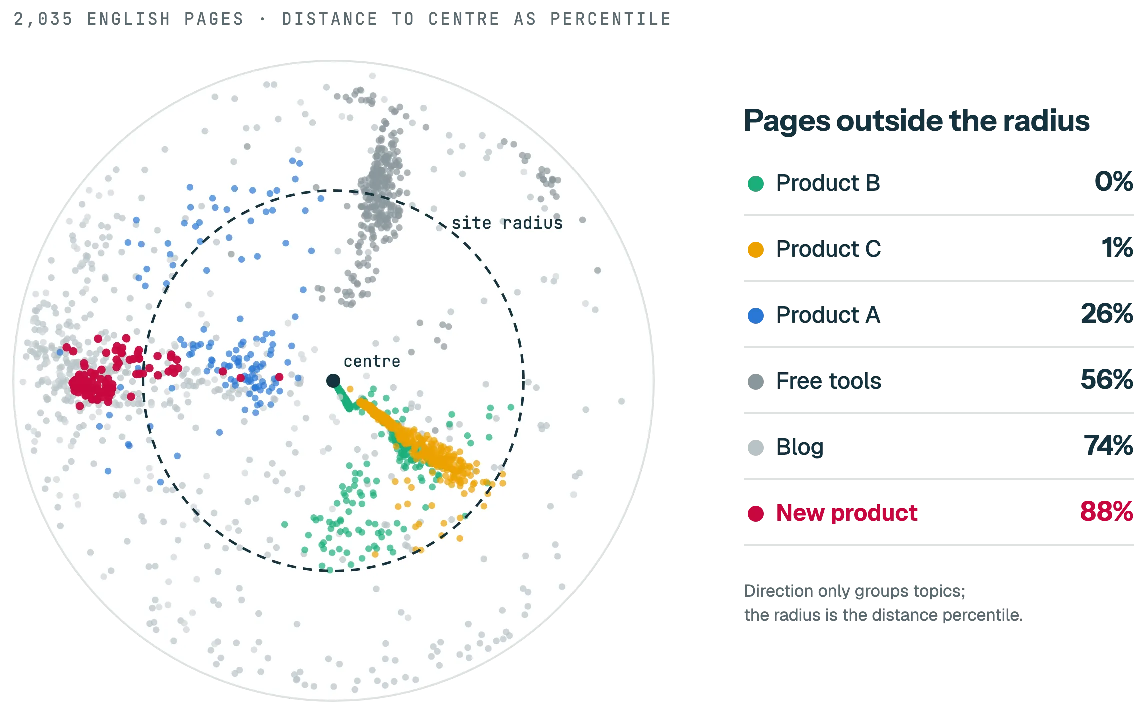
Page type	Pages in English	Outside the radius	Median percentile
Product B	385	0%	10
Product C	441	1%	27
Product A	133	26%	36
Free tools	324	56%	63
Blog	543	74%	80
New product	111	88%	76
Other pages	98	69%	85

What you can see:

The centre of the site is templates. Products B and C have hundreds of pages generated from one template, one for each combination of options. They are almost identical to each other and fill the centre. The centre of the site is where its templates pile up (41% of the URLs in English), and here that doesn’t match what the company wants to sell.

The new product lives at the edge. 88% of its pages fall outside the radius, and its main page is further away than 80% of the site.

The only new product pages that get in are bridges. Of 111, only 13 are inside the radius, and the closest to the centre are use cases that share vocabulary with product A. That type of page is what brings a new topic closer to the centre of a site.

Links don’t explain the problem. With the centre weighted by internal PageRank, the new product holds 11% of the site’s PageRank, and only 8% of that PageRank is outside the radius. The site links to its new product. What it lacks is content that talks about the same things as the rest of the site.

The radius doesn’t explain everything. 56% of the free tools pages are outside the radius, yet they’re still the site’s second-biggest category by estimated traffic (15%), behind only product C. Authority and search intent carry weight too, and the radius can’t see them.

To know whether 88% is a lot, I ran the same calculation on three competitors. Since I only had the full text of the analysed site, for all four I used titles, meta descriptions and H1 to H3 headings, with up to 800 pages per competitor. On all four sites I used the same rule to tag new product pages: the ones that mention it in the URL or the title. That is why the analysed site comes out at 81% outside and not 88%: the text (headings only), the translations and which pages count as the new product all change.

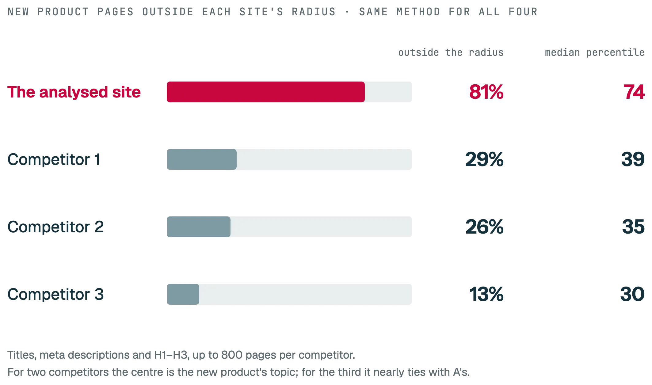
For two of the three competitors, the centre of the site is clearly the new product’s topic; for the third, it almost ties with product A’s. For all three, between 13% and 29% of those pages fall outside the radius. On the analysed site it is the other way round: the new product sits on the periphery.

How many pages do you need to gain relevance?

When a product doesn’t rank, the usual diagnosis is “you lack relevance”, followed by keyword research and a list of content. With embeddings you can be much more specific: which page types to publish, how they need to talk and, above all, how many pages it takes to move the centre of the site.

The process has three pieces:

1. Keyword research for the product. I do it with some AI skills I’ve built, which I’ll share later.
2. The page types competitors rank with for those keywords: comparisons, integrations, use cases, templates.
3. The embeddings, to measure where those pages would fall relative to the centre of your site and simulate how many are needed for the new product to enter the radius.

In the example, I ran the simulation with what was already there: giving more weight to the new product’s current pages, as if it had between 50 and 1,000 more pages like the ones it already has, and recalculating the centre and the radius each time. I did it on the 2,035 pages in English, each counted once. If you count each translation as a URL, what matters is the total number of new URLs: you need about 3,000 for the new product to drop from 85% to 38%. That is, for example, the same 300 pages translated into about 10 languages.

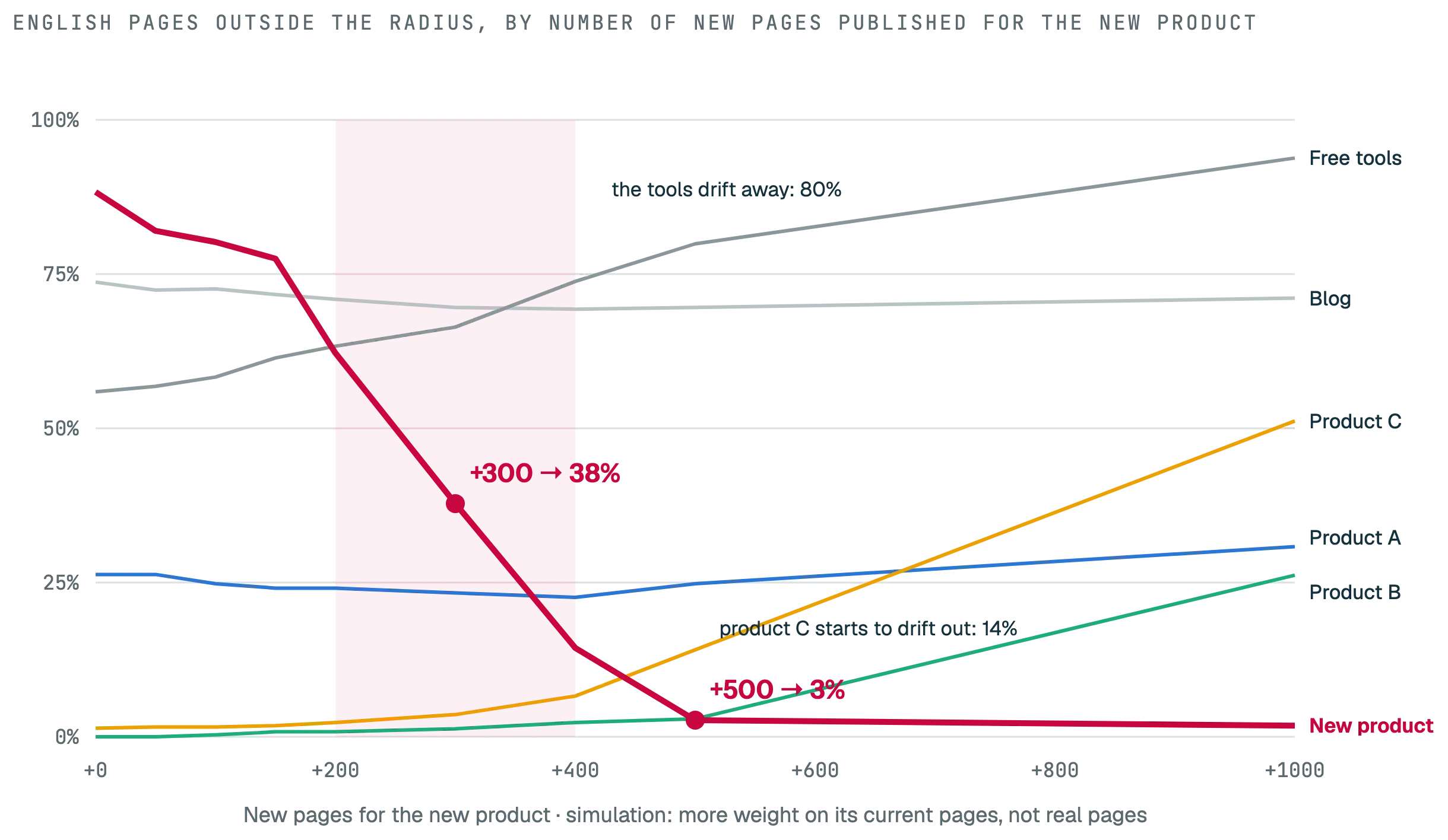
New pages in English	New product outside	Tools outside	Product C outside
0	88%	56%	1%
+200	62%	63%	2%
+300	38%	66%	4%
+400	14%	74%	7%
+500	3%	80%	14%
+1,000	2%	94%	51%

With this model, from about 300 new pages in English most of the new product’s pages end up inside the radius. And there are two more things. The first is that the curve doesn’t fall gradually. Between 200 and 400 pages, the new product goes from 62% to 14%: that’s the point where the site’s centre shifts.

The second seems to me the most useful part of the exercise. The centre moves towards what you publish, and what was close to the previous centre drifts away. With 500 pages, the free tools go from 56% to 80% outside and product C starts to drift out. It is the same mechanism that sinks a website when it opens a section far from its focus, seen from the other side. Publishing a lot of something new also pushes what you already had outside the radius.

The limitations matter:

• The simulation is circular. It models the new pages as copies of the new product’s current ones, and two out of three are per-language template pages that are almost identical to each other. Real pages (templates, comparisons, use cases) will fall somewhere else.
• The right way is to model the pages you are going to publish. Use the competitor pages that rank for your keywords as a model or, better still, a pilot of 20 of your own pages: calculate their vectors, see where they fall and repeat the simulation with the weight of the 300 you plan to publish.
• The jump between 200 and 400 is a cliff. Small changes in the number of pages move the percentage a lot. For a quarterly target it’s a treacherous number.

What are its limits?

What you calculate this way is not Google’s siteRadius. It is a proxy to visualise the relevance of a site: which pages and which page types drift away from the topic set by the rest. It works for that, as long as you’re clear about its limits:

• The model is not Google’s. We don’t know which model Google uses or what text of each page it feeds it, and, as we saw, at least one of its two numbers measures something else. The absolute value won’t resemble Google’s. What you can read is the order: what is closer to the centre and what is further.
• It changes with every decision. The model, the text that goes in (the 30% rule), how many chunks you use per page and how you weight the pages all move the centre. In the example, the new product goes from the 80th to the 21st percentile just by changing the weight. That’s why I work with percentiles and only compare results obtained with the same method.
• The centre is set by volume. The mean goes towards whatever has the most pages. In the example, towards the template pages that are almost identical to each other. Outside the radius means far from what you publish most, which is not necessarily what you sell.
• There are things it doesn’t see. Translations inherit the vector of the original, so a bad translation goes unnoticed. And the distance says what a page is about, but not whether it’s good.
• It’s a correlation. That the new product sits far from the centre fits with it not ranking, but doesn’t prove it.

What do I do with this?

I use it to diagnose and to decide before publishing. Like this:

1. Calculate it by page type. It’s the same logic I use in an SEO audit: the site number is of little use. The percentage outside the radius and the percentile of each page type tell you which parts of the site are far from what the site is.
2. Simulate before opening a section. If you’re going to launch a new page type, measure where it falls and what it pushes outwards.
3. If a section ends up far away, you have three ways out. Add bridges between what you already are and what is new, consolidate the weak pages or split the section into its own subdomain or domain, as we did with the languages at Softonic. If the section is languages, also look at how your international SEO is set up.
4. Don’t use it as a KPI. Merging 50 almost identical pages moves the percentage without gaining anything, and the cliff in the simulation means a target like “less than 40% outside” depends on a dozen pages.
5. Compare competitors only with the same method. Same model, same prefix, same chunking and same type of text. Otherwise you’re comparing preprocessing.

What makes me think this matters is a sentence from Google about site reputation abuse, from November 2024:

Look at the start: “aside from site reputation abuse issues”. The post is about third-party content hosted on reputable sites, but this part talks about something general. Google detects sections that are very different from the main content and measures them as if they were separate sites. And it goes on: those sections can see traffic changes if they “no longer benefit from site-wide signals”, which doesn’t mean they’re penalised: “It means we’re measuring them independently, even if they are located within a site”.

In August 2026 Google updated that policy, which it now calls the site reputation policy, and its documentation says it more directly. Google presumes that “individual pages (including new pages) match the overall quality of other pages on the domain”, and when it separates a part of the site, “over time, our ranking systems learn to rank these parts of a site independently”. There it talks about quality and about sections with third-party content that it separates after a manual review. Even so, it confirms two things that matter here: by default a page inherits the signals of its domain, and a section that Google separates loses them over time.

That the radius in the leak is part of those systems is my own deduction. But if a section of yours sits very far from the centre, the prudent thing is to assume it may not inherit the benefits of the rest of the site.

Who else has calculated it?

I’m not the first, and each person has done it differently:

• Screaming Frog, since version 22, flags “Low Relevance Content” with the same method: it averages the embeddings of all the crawled pages to get a centroid and measures the distance of each page. By default it uses a threshold of 0.4 and gets the vectors from OpenAI, Gemini or Ollama. In the version 22 announcement they link it to the leak: measuring how far page embeddings deviate from the site embedding “was hinted at within the Google leak”.
• DEJAN has a Space on Hugging Face, now paused (the code can be read), with the LaBSE model. It uses the slugs of the URLs in the sitemap instead of the text of the pages.
• Patrick Stox has a Semantic Site Map with all-MiniLM-L6-v2 on the article text and topics by spherical k-means, with a radius per topic. He warns that distances “only have meaning within this site’s included corpus”.
• Taha Yelkenci calculates it with TF-IDF instead of embeddings, and also makes it clear: his radius says nothing about Google’s siteRadius.
• Eric Gilley, at iPullRank, used it to prune a blog of more than 1,000 posts: topic centroids from keywords, plus a vector with the business description, combined with Search Console clicks and post age. They flagged close to 45% of the posts and removed or redirected more than 500.
• Go Fish Digital offers a semantic audit that says it starts from the leak and measures a “Focus Score” and a “Site Radius”. It doesn’t publish how it calculates them.
• Gus Pelogia explained on the Screaming Frog blog how to get embeddings from a crawl and calculate similarities between pages, which is the starting point for all of this.

What this post adds: cutting the text of each page into chunks and averaging them (DEJAN uses only the URL slug), translations handled through hreflang, the comparison of weightings, the simulation and what it means that focus and radius come out the same.

The script

The snippets for each step are above. I’ll email you the full script, the one that reads the CSV (with the weights you pass it), splits the text, calculates distances and percentiles and produces the summary by page type, along with a README and a sample CSV.

It needs a CSV with two required columns, url and text, and two optional ones: group (the page type, the product or whatever you want to compare) and weight (internal PageRank, traffic or whatever you want to use as a weight). It accepts CSV separated by commas, semicolons or tabs, in UTF-8. Be careful with weights: if you weight by traffic, a few URLs set the centre and almost the whole site ends up outside the radius. Use it to see what pulls on the centre, not to read the percentage outside.

Any crawler works for extracting the text. The important thing is to leave out the menu, footer and banners: configure the extraction to take only the main content, or apply the 30% rule from step 1.

It runs on CPU, with no GPU or API keys. The first time it runs, it downloads the model (a few hundred MB). If you want to try another one, pass it with --model and, if its model card asks for a prefix, add it with --prefix.

Here’s the output for the example’s 2,035 pages, with the groups already anonymised. The figures match the example table (English pages, every URL weighted equally):

2035 pages · site radius 0.0306 · focus 0.9694
90th percentile of distance 0.0481 · standard deviation 0.0132
group                  pages outside percentile
product-b                385      0%       0.10
product-c                441      1%       0.27
product-a                133     26%       0.36
tools                    324     56%       0.63
new-product              111     88%       0.76
blog                     543     74%       0.80
other                     98     69%       0.85

The output CSV has one row per page, sorted from the closest to the centre to the furthest, with its distance, its percentile and whether it falls outside the radius. Open it and start from the end: that’s where the pages that fit your site least are.

References

1. Google Content Warehouse API: QualityAuthorityTopicEmbeddingsVersionedItem . HexDocs
2. Google Content Warehouse API: CompressedQualitySignals . HexDocs
3. Google Content Warehouse API: QualityNsrNsrData . HexDocs
4. Mike King. Secrets from the Algorithm: Google Search’s Internal Engineering Documentation Has Leaked . iPullRank (2024-05-28)
5. Mia Sato. Google confirms the leaked Search documents are real . The Verge (2024-05-29)
6. A guide to Google Search ranking systems . Google Search Central
7. Chris Nelson. What creators should know about Google's August 2022 helpful content update . Google Search Central (2022-08-18)
8. Creating helpful, reliable, people-first content . Google Search Central
9. Chris Nelson. Updating our site reputation abuse policy . Google Search Central (2024-11-19)
10. Update to the Site Reputation Policy . Google Search Central (2026-08-28)
11. Spam policies for Google web search: site reputation policy . Google Search Central (2026-08-28)
12. Jen Granito. Understanding news topic authority . Google Search Central (2023-05-23)
13. Danny Sullivan. Danny Sullivan on covering several topics on one blog . Mastodon (2022-12-11)
14. Danny Sullivan. Danny Sullivan on the topics line in the 2022 post . Mastodon (2022-12-11)
15. John Mueller. John Mueller on unrelated content on a site . Bluesky (2025-06-10)
16. Yevgen Tsykynovskyy. US20200050707A1: Website representation vector . Google Patents (2020-02-13)
17. Bill Slawski. Google Using Website Representation Vectors to Classify with Expertise and Authority . Go Fish Digital (SEO by the Sea archive) (2020-02-21)
18. David Gehrking, Ching Law, Andrew Maxwell. US8229957B2: Categorizing objects, such as documents and/or clusters, with respect to a taxonomy . Google Patents (2012-07-24)
19. Navneet Panda, Vladimir Ofitserov, Kaihua Zhu. US9684697B1: Ranking search results . Google Patents (2017-06-20)
20. April R. Lehman, Navneet Panda. US9031929B1: Site quality score . Google Patents (2015-05-12)
21. Navneet Panda, Yun Zhou. US9767157B2: Predicting site quality . Google Patents (2017-09-19)
22. Nissan Hajaj. US9165040B1: Producing a ranking for pages using distances in a web-link graph . Google Patents (2015-10-20)
23. Brian Patrick Strope, Quoc V. Le. US9984062B1: Generating author vectors . Google Patents (2018-05-29)
24. Amit Singhal, Urs Hölzle. US8595225B1: Systems and methods for correlating document topicality and popularity . Google Patents (2013-11-26)
25. US10235423B2: Ranking search results based on entity metrics . Google Patents (2019-03-19)
26. Michael J. Procopio. US8458196B1: System and method for determining topic authority . Google Patents (2013-06-04)
27. Krishna Bharat, George A. Mihaila. When Experts Agree: Using Non-Affiliated Experts to Rank Popular Topics (Hilltop) . WWW10 (2001)
28. Taher H. Haveliwala. Topic-Sensitive PageRank . WWW 2002 (2002)
29. Quoc V. Le, Tomas Mikolov. Distributed Representations of Sentences and Documents . Google (arXiv) (2014)
30. Daniel Cer et al.. Universal Sentence Encoder . Google (arXiv) (2018)
31. Jianmo Ni et al.. Sentence-T5: Scalable Sentence Encoders from Pre-trained Text-to-Text Models . Google (arXiv) (2021)
32. Jianmo Ni et al.. Large Dual Encoders Are Generalizable Retrievers . Google (arXiv) (2021)
33. Jinhyuk Lee et al.. Gecko: Versatile Text Embeddings Distilled from Large Language Models . Google DeepMind (arXiv) (2024)
34. Jinhyuk Lee et al.. Gemini Embedding: Generalizable Embeddings from Gemini . Google (arXiv) (2025)
35. Gemini Embedding 2: A Native Multimodal Embedding Model from Gemini . Google (arXiv) (2026)
36. EmbeddingGemma 2: Unified and Efficient Multimodal Representations . Google (arXiv) (2026)
37. H. Schechter Vera et al.. EmbeddingGemma: Powerful and Lightweight Text Representations . Google (arXiv) (2025)
38. Liang Wang et al.. Text Embeddings by Weakly-Supervised Contrastive Pre-training . Microsoft (arXiv) (2022)
39. Liang Wang et al.. Multilingual E5 Text Embeddings: A Technical Report . Microsoft (arXiv) (2024)
40. intfloat/multilingual-e5-small . Hugging Face
41. Sylvain Lugeon, Tiziano Piccardi, Robert West. Homepage2Vec: Language-Agnostic Website Embedding and Classification . EPFL (arXiv) (2022)
42. J. Gerber, J. Saxer, B. Kreiner, A. Weiler. Benchmarking state of the art website embedding methods for effective processing and analysis in the public sector . Journal of Intelligent Information Systems (2025)
43. Harald Steck, Chaitanya Ekanadham, Nathan Kallus. Is Cosine-Similarity of Embeddings Really About Similarity? . Netflix (arXiv) (2024)
44. Directional statistics . Wikipedia
45. Dan Sharp. Screaming Frog SEO Spider Update – Version 22.0 . Screaming Frog (2025-06-10)
46. How to Identify Semantically Similar Pages & Outliers . Screaming Frog
47. siteFocusScore (Hugging Face Space) . DEJAN
48. Patrick Stox. Semantic Site Map
49. Taha Yelkenci. How to Audit Your Site Against the Google Leak Signals (2026-10-15)
50. Eric Gilley. Relevance Engineering at Scale: Smarter Content Pruning with Embeddings & SEO . iPullRank (2025-05-14)
51. Semantic Content Audit . Go Fish Digital
52. Gus Pelogia. Using the Screaming Frog SEO Spider and OpenAI Embeddings to Map Related Pages at Scale . Screaming Frog (2024-09-23)